In many applications, we not only need the classification result from Transformer, but also need to explain the model’s behavior: how the Transformer makes decisions, which input features the Transformer model uses to make output (classification) decisions, or the contribution of input features to Transformer output. This requires us to explore Explainability in Transformer.
So in this blog, I’ll focus on explaining the Transformer model’s behavior. We first discuss the most popular method – the Attention-based method, which is applicable to both Vision and Language models. And then I’ll talk about some special methods for explaining the Vision model (Vision Transformer) – applying the explanation method in CNN to Transformer.
1. Attention-based method
1.1 Raw attention
Recap that, in the self-attention mechanism, the output is the weighted sum of input:
\[A=softmax(\frac{Q·K^T}{\sqrt{d_h}})\]
\[O=A·V\]
More specifically, the output \(y_i\) of a token \(i\) is computed as a weighted sum of all input tokens, where the weights \(\alpha_{ij}\) are given by the attention matrix \(A\) :
\[y_i = \sum_{j}^{}{\alpha_{i,j} v_j}\]
So intuitively, we can use these weights \(\alpha_{ij}\) from attention matrix \(A\) to quantify how important is the input tokens to output tokens, where each row corresponds to a relevance map for each token given the other tokens.
Since we focus on classification models, only the [CLS] token, which encapsulates the explanation of the classification, is considered. The relevance map is, therefore, derived from the row \(C_{[CLS]} \in R_s\) that corresponds to the [CLS] token. This row contains a score evaluating each token’s influence on the classification token:
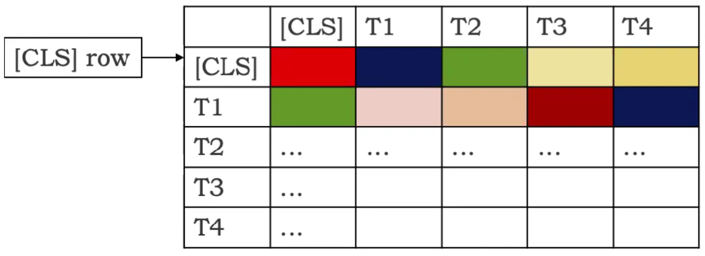
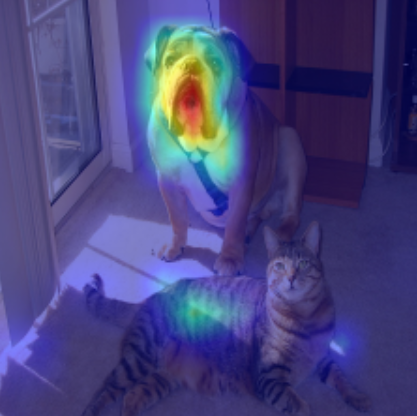
Typically people use the last layer’s attention matrix (yields better results). It’s a vector of 1*197 dim. And we discard the first element (it’s the importance of [CLS] token to [CLS] token; not so important) to get a 1*196 dim vector. For vision model, to visualize it like an image, we can first reshape it into a 14*14 matrix to get a token level explanation. But we care about pixel-level explanation, so what we typically do is use bilinear interpolation to upsample it into a 224*224 image (Same size as the input image. Here we use the ImageNet dataset’s image as an example).
Here’s what we get:
Code:
# Look at the total attention between the class token, and the image patches
mask = A[0, 0 , 1:]
# In the case of the 224x224 image, this brings us from 196 to 14 (width=14)
width = int(mask.shape[-1]**0.5)
mask = mask.reshape(width, width).numpy()
mask = mask / np.max(mask)
# resize到与image尺寸一样,即可得到saliency map
mask = cv2.resize(mask, (image.shape[-1], image.shape[-2]))
plt.imshow(mask)
Simply visualizing the raw attention matrix is the most popular method. It’s very easy to implement, and yet yield intuitive result.
But often the visualizing result is not so ideal, either too noisy or not highlighting the truly important region. The nice results in the paper are often carefully chosen and could not reflect the general explanation performance. A better explanation method is needed.
But how? One direction is exploiting more information from the Transformer model. We have more attention maps from multiple heads and layers, right? Let’s use it to aggregate multiple attention matrices from many heads and layers. But here are some difficulties:
Many heads are useless – if we prune most of the heads, then the performance will not be affected…
So we can not treat these heads as equal when calculating the saliency map.
- (2) Many attention layers
Attentions are combining non-linearly from one layer to the next.
Successful explanation methods must have their own way to solve these difficulties.
1.2 Attention Rollout [1]
The Attention rollout method makes a few assumptions to simplify the problem:
- (1) Head aggregation by average
It assumes all heads are equal, so we can just average over them:
\[E_h A^{(b)} = \frac{1}{M}\sum_{m}^{}{A_m^{(b)}}\]
(here “b” means block b)
- (2) Layer (Block) aggregation by (attention) matrix multiplication
It assumes attentions are combined linearly – self-attention layers are stacked linearly one after another, and another mechanism (like FFN) does not make any changes to how the model uses input features to make decisions.
But residual connection matters. So we can model it as \(\hat{A}^{(b)}=I+E_h A^{(b)}\)(you can see it as \(y_i = y_i+\sum_{j}^{}{\alpha_{i,j} v_j}=(1+\alpha_{ii})y_i+\sum_{j\ne i}^{}{\alpha_{i,j} v_j}\)), and then normalize it to make each row sum up to 1 again: \(\hat{A}^{(b)}= \hat{A}^{(b)} / \hat{A}^{(b)}.sum(dim=-1)\) .
And then use matrix multiplication to aggregate across layers:

This is because we model the attribution of token \(i\) at block \(b\) to token \(j\) at block \(b+1\) as:
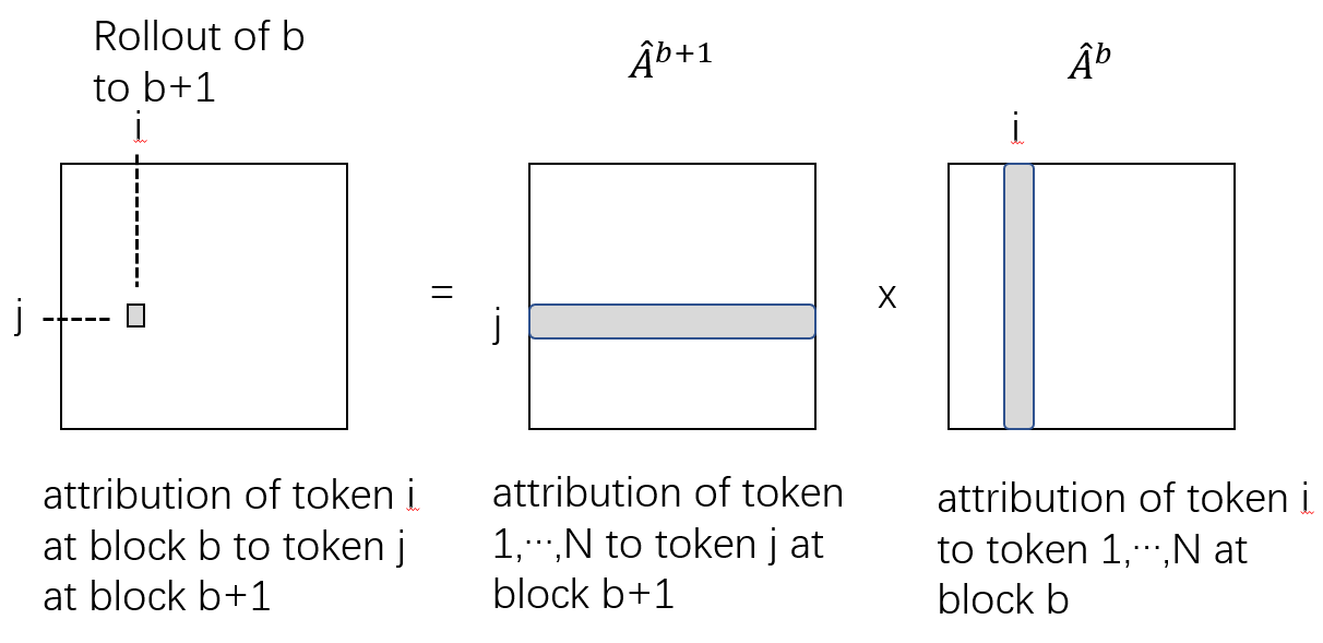
To make the assumptions of (1) and (2) more realistic, [2,3] propose a few improvements:
- (1) Head aggregation by weighted sum
[4] Observe that different heads attend to different objects or parts:
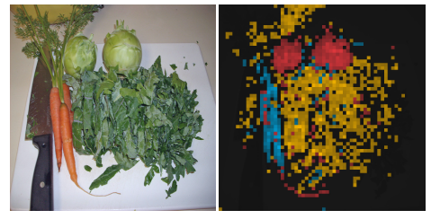
(Picture: Visualization of attention map of each head with different color)
As each head attends to different information, each head should have different importance for different output class predictions. For example, in the plot above, if we want to explain which part of an input image is used by the model to predict class “carrot”, then we want only the blue part to be highlighted, so the attention matrix that corresponds to the blue part should have highest weight. And if we average them like what we did in Attention Rollout, we might get a saliency map highlighting all objects rather than the object we want to explain to.
So to explain a specific class, we should weigh the heads and these weights should be related to the class. This motivates us to choose gradient as weight:
\[E_h A^{(b)} = \frac{1}{M} \sum_{m}^{} ∇A_m^{(b)}\odot A_m^{(b)}\]
, where \(\ ∇A_m^{(b)} = \frac{\partial y_c}{\partial A_m^{(b)}}\), and c is the class we want to explain to.
(Other choices of aggregation, like taking the minimum, or taking the maximum, don’t enable a class-specific signal.)
Besides, since we only care about which part is used to make a decision, the positive contribution is considered. So we can discard the negative part in the attention matrix:
\[E_h A^{(b)} = \frac{1}{M} \sum_{m}^{} ∇A_m^{(b)} \odot A_m^{(b)+}\]
- (2) Layer (Block) aggregation by (attention) matrix multiplication
Same as before.
Note that in [2] authors use relevance score R (calculated from LRP method) to replace raw attention matrix A, but later in [3] they find out that it’s not so helpful, so they use attention matrix A again.
Code:
# attentions has shape [layer, batch, channel, H, W]
# Without LRP
result = torch.eye(attentions[0].size(-1))
with torch.no_grad():
  for attention, grad in zip(attentions, gradients):
	   weights = grad
	   attention_heads_fused = (attention*weights).mean(axis=1)
	   attention_heads_fused[attention_heads_fused < 0] = 0

	   I = torch.eye(attention_heads_fused.size(-1))
	   a = (attention_heads_fused + 1.0*I)/2
	   a = a / a.sum(dim=-1)
	   result = torch.matmul(a, result)
1.4 Aggregation methods as hyperparameters
Previously we talk about many ways to aggregate attention matrix. But the results of GAE are not necessarily the best. For example, Sometimes it’s better to aggregate the attention matrix from the last layer to 4 th layer is better than to the first layer, but sometimes it’s worse. So [5] Propose that the ways of aggregation can be hyperparameters:
ways of aggregating over multiple heads, and layers:
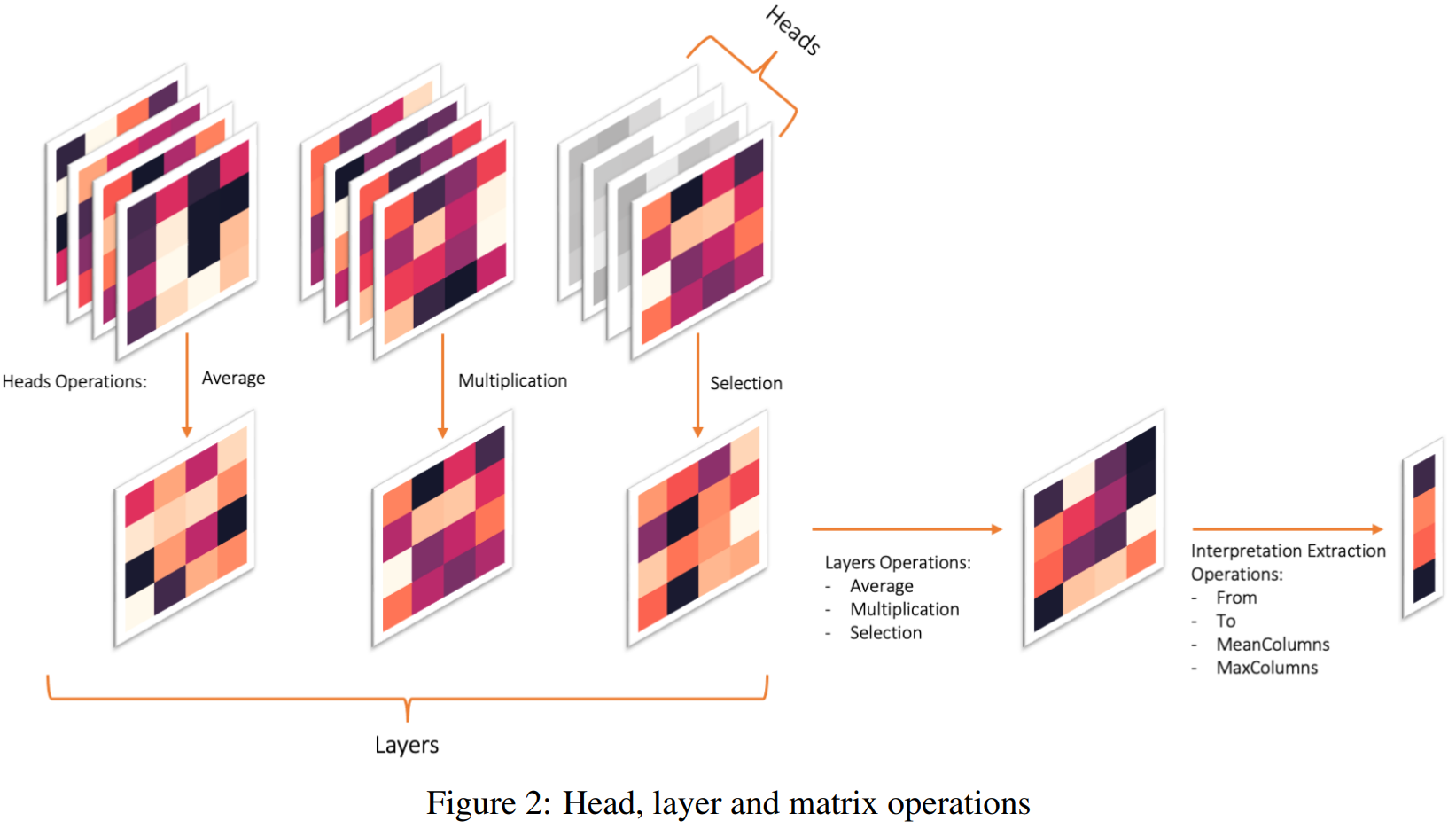
And for each hyperparameter, we evaluate its result and choose the one that yields the best evaluation results.
But it’s computationally costly to search over those hyperparameters (because we have to evaluate them many times), so people still prefer using GAE as default.
1.5 Norm-based methods [6]
[5] Observe that although some tokens might have large attention weights \(\alpha_{ij}\), their value vector \(f(x_j)\) is actually very small, so overall it has a small contribution.

So instead of using attention weights \(\alpha_{ij}\) as attribution of token \(j\) to token \(i\) , they propose to use the norm \(\|\|\alpha_{ij}f(x_j)\|\|\) . And then we can aggregate over heads and layers as we did in 1.3.
1.6 Limitation
(1) Too much simplification:
- ignore FFN and negative components in each attention block.
- ignore non-linearity in self-attention.
(2) Ongoing debate about attention as a faithful explanation.
There’s a debate about whether attention is a faithful explanation. Some of their observations are: attention attribution is not correlated well with other explanation methods’ results, and randomly perturbing attention does not affect the model’s prediction, which all indicates attention is not a faithful explanation [7].
But [8] provides a possible answer to why discarding learned attention patterns have a low impact: most parts of token information are preserved by residual connection:
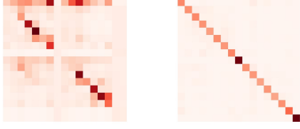
(This is the visualization of the attention map before (left) and after (right) adding a residual connection. The right one is diagonal, which means the tokens itself has the highest contribution to themselves)
So only perturbing attention does not change too much, if they don’t change residual connection.
Previously we talked about the Attention-based method, which is uniquely designed for Transformers because it uses a unique element of the attention map.
But before Vision Transformer (ViT) was proposed, there were already many explainability methods for CNN, including gradient-based, CAM-based (feature-based), and perturbation-based methods. All of them can be modified and applied to explain the Transformer model.
2.1 Gradient-based method
We can use Input gradient, Smoothgrad, and Integrated Gradient in the exact same way as we use in CNN.
Similar to CNN’s explanation, we also get a very noisy visualizing result.
And for ViT, I also observe a strong checkboard artifact (discontinuity between neighboring patches) from visualizing the result:
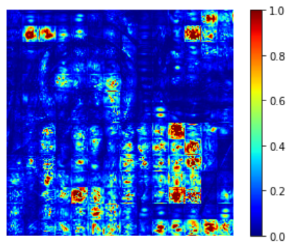
It probably stems from the strided convolutions in ViT (we use strided convolutions as a way to combine cutting image into patches+linear transformation).
For more about strided convolutions causing checkboard artifacts, see: https://distill.pub/2016/deconv-checkerboard/
2.2 CAM-based (feature-based) method
(1)Grad-CAM
We can extract feature maps as follows [9]:
In ViT the output of the layers is typically BATCH x 197 x 192. At dimension 197, the first element represents the class token, and the rest represents the 14x14 patches in the image. We can treat the last 196 elements as a 14x14 spatial image, with 192 channels.
Since the final classification is done on the class token computed in the last attention block, the output will not be affected by the 14x14 channels in the last layer. The gradient of the output with respect to them will be 0!
We should choose any layer before the final attention block, for example:
target_layers = [model.blocks[-1].norm1]
And Gradients can be calculated easily using backprop. We use gradient as weights of features, and then Combine those two terms, we get Grad-CAM.
(2) ViT-CX [10]
We first extract feature maps as above.
But instead of using gradient as weight, we first apply feature maps as masks M to perturb input $X$, and then the output is the weight.

Here $Rd$ is a matrix of random numbers, which has the same size as the feature map
The intuition is, if the feature map highlights the important region of the input image, then retaining this region by \(X\odot M_I\) and masking another region out (or blur it with \(Rd\odot(1-M_i)\) ) will yield a high output classification score.
2.3 Perturbation-based method
(1) Value Zeroing [11]
Perturbation-based method aims to measure how much a token uses other context tokens to build its output representation \(\tilde{x}_ i\) at each encoder layer by perturbing the input token.
In Value Zeroing, to measure attribution of input token \(i\) to output token \(j\) , it zeros the input value vector of token \(i\) when calculating the output of token \(j\) :
\[output: \ z_i^h=\sum_{j=1}^{n}{\alpha_{i,j}^h v_j^h} , \ and \ set \ v_j=0\]
This provides an alternative output representation \(\tilde{x}_ i^{-j}\). And then measure how much output changes by:
\[C_{i,j} = \tilde{x}_ i^{-j} * \tilde{x}_ i\]
where the operation ∗ can be any pairwise distance metric (eg. cosine distance).
The intuition is, if input token \(i\) is important to output token \(j\) , then masking input token \(i\) out will make \(\tilde{x}_ i\) change a lot and yield a large distance between \(\tilde{x}_ i\) and \(\tilde{x}_ i^{-j}\).
For all input token \(i\) and output token \(j\) , we can calculate \(C_{i,j}\) as above, generating a map similar to attention map. And then we can aggregate over layers and heads as before.
2.4 Activation Maximization
Optimize over input image to maximize the output of a “unit” \(S_c(I)\) (can be mean of a layer or token) in Transformer:
\[argmax_I \ S_c(I)-\lambda ||I||^2_2\]
The second term is a spatial regularization term (to make the result smoother). The results also have checkboard artifact:
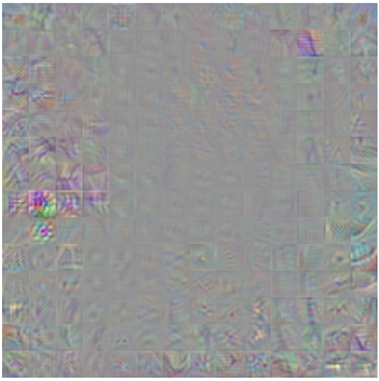
Instead of getting a continuous image, we get 14x14 patches, many neighboring patches look similar, but they also have a discontinuity between them [8].
3. Useful resources
[1] A great talk by Hila Chefer for attention-based method: Hila Chefer - Transformer Explainability
[2] A good tutorial: https://github.com/jacobgil/vit-explain
4. Reference
[1] Samira Abnar, Willem Zuidema. 2020. Quantifying Attention Flow in Transformers.
[2] Hila Chefer, Shir Gur, and Lior Wolf. 2021. Generic Attention-model Explainability for Interpreting Bi-Modal and Encoder-Decoder Transformers.
[3] Hila Chefer, Shir Gur, and Lior Wolf. 2021. Transformer Interpretability Beyond Attention Visualization.
[4] Mathilde Caron, Hugo Touvron, Ishan Misra, Herve Jegou, Julien Mairal, Piotr Bojanowski, Armand Joulin. 2021. Emerging Properties in Self-Supervised Vision Transformers.
[5] Nikolaos Mylonas, Ioannis Mollas, and Grigorios Tsoumakas. 2022. AN ATTENTION MATRIX FOR EVERY DECISION: FAITHFULNESS-BASED ARBITRATION AMONG MULTIPLE ATTENTION-BASED INTERPRETATIONS OF TRANSFORMERS IN TEXT CLASSIFICATION.
[6] Goro Kobayashi, Tatsuki Kuribayashi, Sho Yokoi, Kentaro Inui. 2020. Attention is Not Only a Weight: Analyzing Transformers with Vector Norms. Proceedings of the 2020 Conference on Empirical Methods in Natural Language Processing, pages 7057–7075.
[7] Adrien Bibal, Rémi Cardon, David Alfter, Rodrigo Wilkens, Xiaoou Wang, Thomas François∗ and Patrick Watrin. 2022. Is Attention Explanation? An Introduction to the Debate. Proceedings of the 60th Annual Meeting of the Association for Computational Linguistics Volume 1: Long Papers, pages 3889 - 3900.
[8] Goro Kobayashi, Tatsuki Kuribayashi, Sho Yokoi, Kentaro Inui. 2021. Incorporating Residual and Normalization Layers into Analysis of Masked Language Models. Proceedings of the 2021 Conference on Empirical Methods in Natural Language Processing, pages 4547–4568.
[9] Jacob Gildenblat. pytorch-grad-cam/vision_transformers.md at master · jacobgil/pytorch-grad-cam · GitHub
[10] Weiyan Xie, Xiao-Hui Li, Caleb Chen Cao, and Nevin L. Zhang. 2022. ViT-CX: Causal Explanation of Vision Transformers.
[11] Hosein Mohebbi, Willem Zuidema, Grzegorz Chrupała, and Afra Alishahi. 2023. Quantifying Context Mixing in Transformers.