1.Background: What is End-to-End Motion Prediction in Autonomous driving
Traditionally the whole working pipeline of autonomous driving is the modular pipeline, which consists of four separate modules: perception, prediction, planning, and control [4]:

But it suffers from some drawbacks, like pice-wise training, and non-shared computation and information. So the recent trend is developing in an end-to-end fashion, which jointly develops perception and prediction modules:

It has two key advantages: (1) shared computation and (2) shared information between modules.
The working pipeline of end-to-end motion prediction is as follows:
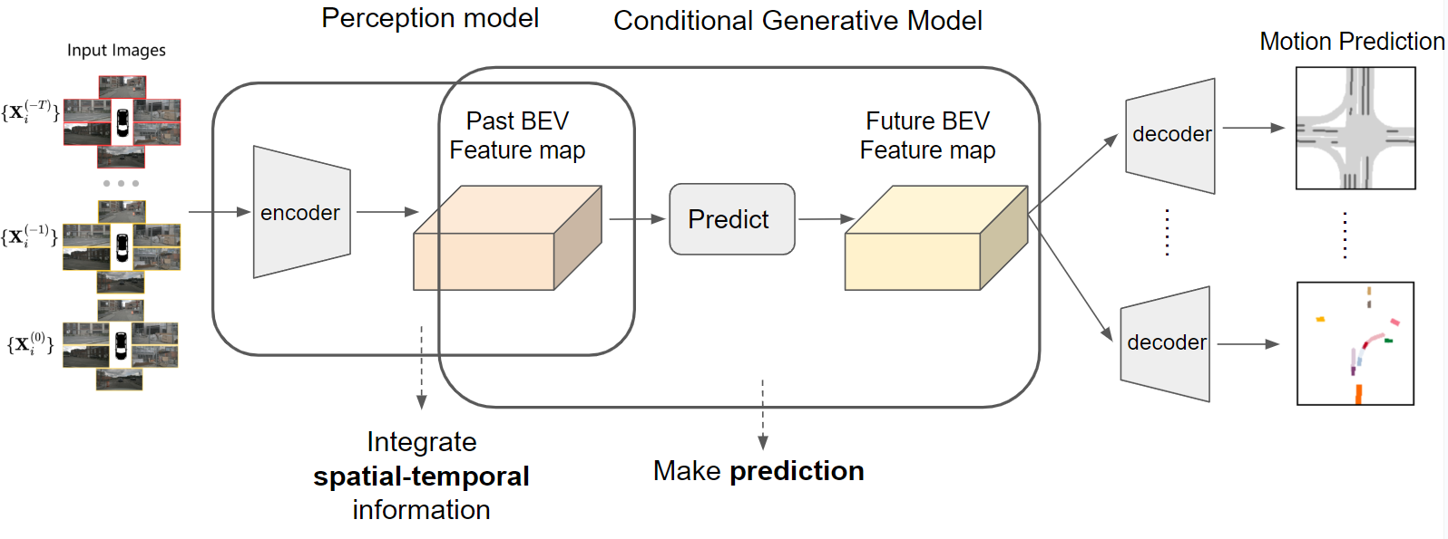
As you can see, there’re three key components here, perception model, conditional generative model, and prediction heads.
First, we have a perception model that encodes information into past BEV feature maps from past sensor input, and then we have a conditional generative model that generates future BEV feature map condition on the past BEV feature map (which we will elaborate on next), and then several prediction heads are employed to decode them for future motion prediction tasks.
The perception model is pretty much similar to those models for perception-only tasks like BEVFormer [3], and actually, if you employ several decoder heads for the past BEV feature maps, you will get perception results, so I won’t spend too much time talking about it. And the prediction heads are just usual detection heads, and segmentation heads, so we can directly use the existing model. The new thing is the conditional generative model, which is borrowed from the prediction-only task but is modified a little. So in this blog, I will focus on introducing the conditional generative model.
2.Probabilistic prediction framework
We can model the prediction mechanism as a conditional probability distribution \(P (Y |S) = p(y_1, · · ·, y_{T'} |s_1, · · ·, s_T )\) that generates T’ future state feature \(Y = \{y_1, y_2, · · ·, y_{T'} \}\) given past state features for each frame \(S = \{s_1, s_2, · · ·, s_T \}\) or a single state feature \(S=s\) that represent all past frames, which are extracted from sensor data or/and HD maps.
Once we have an explicit form of this conditional probability distribution, we can sample future BEV features \(Y\) from it \(Y~P (Y |S)\) and feed it to prediction heads.
But unfortunately, it’s intractable, so we have to add some assumptions to factorize it.
Various factorizations of \(P(Y | S)\) utilize different levels of independence assumptions:
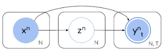
(a) Assume independent futures across time steps, then we get:
\[P(Y |S) = \prod_{t}^{} P(y_t|S)\]
The problem is, the independence assumption does not hold in practice.
(b) Autoregressive generation
\[P(Y |S) = \prod_{t}^{} P(y_t|Y^{0:t-1},S)\]
We assume the next frame depends on previous ones. So we can model \(P(y_t \| Y^{0:t-1}, S)\) as an RNN [5,6] (then we’re back to a deterministic model).
(c) Assume there’s a latent/hidden state that generates future trajectories [1]:
\[P (Y |S) = ∫ _Z P (Y |S, Z) P (Z|S) dZ\]
, where \(Z\) is a latent variable that is assumed to generate future frames. So it must by design capture all future (unobserved) scene dynamics (such as actor goals and style, multi-agent interactions, or future traffic light states).

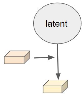

So sampling future BEV features \(Y\) from it \(Y~P (Y \| S)\) is equivalent as a two stages of sampling:
Step 1. Sample a latent code from a latent distribution \(Z ∼ P (Z \| S)\)
Step 2. Sample future BEV feature maps \(Y\) from the conditional generative distribution \(P (Y \| S, Z)\).
The performance of the generation process is intrinsically dependent on two key factors. Firstly, the quality of the latent code is crucial, as it should encompass the necessary future information required for generating the future map. Secondly, the capacity of the generative process plays a vital role, as it enables the effective fusion of past information and latent information to generate the future feature map.
So next, I’ll elaborate on those two factors one by one.
2.1 Latent distribution P(Z|S)
Existing literatures propose two ways of generating the latent variable \(Z\).
(a) A trainable parameter as latent
In [7], they make the latent variable \(Z\) as a trainable parameter. And during training, once the labels of future frames are used (in those prediction tasks), the future information is injected into the latent code, so hopefully, the latent code can be learned to be a latent code that generates the future.
(b) Latent distribution (also called “future distribution in [2]”)
To learn a distribution about latent state \(Z\), we formulate two latent distributions with and without GT future state \(Y_{GT}=(y_{t+1}^{GT}, ..., y_{t+T'}^{GT} )\): \(P(Z \|S)\) and \(P(Z \|S, Y_{GT})\), where \(P(Z \|S)\) is what we actually use for inference (cover all the possible modes contained in the future) and need to be learned, while \(P(Z \|S, Y_{GT})\) additionally take ground truth future state as input and thus is used as supervision for learning \(P(Z \|S)\). And we learn the \(P(Z \|S)\) to approximate \(P(Z \|S, Y_{GT})\).
(For simplicity,) We parametrize both distributions as diagonal Gaussians with mean \(μ \in R^L\) and variance \(σ^2 \in R^L\) which are learnable parameters, \(L\) being the latent dimension: \(P(Z \| S) = N (μ_{t}, σ^2_{ t})\), \(P(Z \| S,Y_{GT}) = N (μ_{t,gt}, σ^2_{t,gt})\).
(1) Latent distribution w/o GT: \(P(Z|S)\): represents what could happen given the past context
- Input past state feature \(S\) that represents the past T frames (as the condition of distribution).
- Transformed \(S\) by a learnable NN (map dim of \(S\) to the desired latent dimension \(L\)).
- Downsampling convolutional layers + average pooling layer + FC
- Two heads for outputing parametrization of the present distribution: \((μ_{t}, σ_{t}) \in R^L × R^L\).
(2) Latent distribution w GT: \(P(Z|S,Y_{GT})\): represents what actually happened in that particular observation.
- Input \(S\), and information about future frames (Gt label/state/latent of future prediction task \(Y_{GT}\), “observed future”)
- Transformed \(S\) and \(Y_{GT}\) by a learnable NN.
- For \(S\): Downsampling convolutional layers + average pooling + FC as before.
- Concatenate output of all time steps, and feed them to another FC.
- Output parametrisation of the present distribution: \((μ_{t,gt}, σ_{t,gt}) \in R^L × R^L\).
Learning the latent distribution
And then we learn by encouraging \(P(Z\|S)\) to mach \(P(Z \| S, Y_{GT})\) by optimizing the following loss (min the KL divergence between two distributions) (or equivalently, optimize ELBO):
\[\text{min} \ D_{KL}(P(S|Z) || P(S|Z,Y_{GT}) )\]
Probabilistic Future Prediction
During training: sample latent future from \(P(Z\|S, Y_{GT})\): \(Z ∼ N (μ_{t,gt}, σ^2_{ t,gt})\), for all future frames prediction.
During inference: sample latent future from \(P(Z \| S)\): \(Z ∼ N (μ_{t}, σ^2_{ t})\) (each sample corresponds to a different possible future).
2.2 Conditional generative distribution P (Y |S, Z)
Starting from the latent code as illustrated in 2.1, through a series of cross-attention mechanisms, future BEV feature maps are generated. Concurrently, the past BEV feature map obtained from the perception model is transformed into keys and values for cross-attention integration, serving as a conditional input to control the generation process.
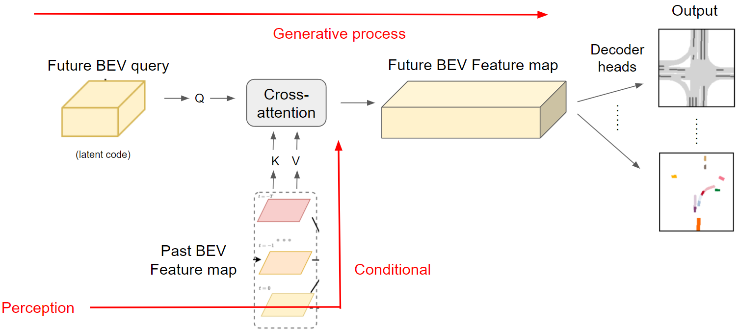
Doesn’t it look familiar with the recent text-to-image generation?
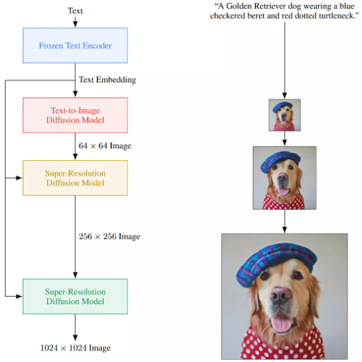
Unfortunately, all current literature didn’t use “real” generative models like GAN, VAE, or diffusion model, but only use a deterministic approach to approximate it (So that’s why my PhD research proposal is to use a real generative model to do that. I’ll elaborate it in another blog).
If we use a deterministic mapping \(Y = f_{predict} (S, Z)\) to implicitly characterize \(P (Y \|S, Z)\) instead of explicitly representing it in a parametric form, we can avoid factorizing \(P (Y \|S, Z)\). In this kind of framework, generating scene-consistent future state \(Y\) (by sample \(Y\) from \(P(Y \|S)\)) is simple and highly efficient since it only requires one stage of sampling:
Step 1. Sample a latent scene from the latent distribution \(Z ∼ P (Z \| S)\)
Step 2. Decode with the deterministic decoder \(Y = f_{predict} (S, Z) \approx P (Y \| S, Z)\).
This is exactly the same as any other deterministic end-to-end motion prediction mechanism \(Y=f_{predict}(X)\), with an additional probabilistic element \(Z\) added, which captures all stochasticity in the generative process.
In [5] and its follow-up papers [6,8], an RNN is used as \(f_{predict}\); and in [7], the decoder part of a Spatio-Temporal Pyramid Network is used as \(f_{predict}\).
Reference
[1] Casas, S., Gulino, C., Suo, S., Luo, K., Liao, R., & Urtasun, R. (2020). Implicit Latent Variable Model for Scene-Consistent Motion Forecasting. ArXiv, abs/2007.12036.
[2] Hu, A., Cotter, F., Mohan, N.C., Gurau, C., & Kendall, A. (2020). Probabilistic Future Prediction for Video Scene Understanding. European Conference on Computer Vision.
[3] Zhiqi Li, Wenhai Wang, Hongyang Li, Enze Xie, Chonghao Sima, Tong Lu, Qiao Yu, and Jifeng Dai. Bevformer: Learning bird’s-eye-view representation from multi-camera images via spatiotemporal transformers. ArXiv, abs/2203.17270, 2022,
[4] Joel Janai, Fatma Guney, Aseem Behl, and Andreas Geiger. Computer vision for autonomous vehicles: Problems, datasets and state-of-the-art. ArXiv, abs/1704.05519, 2017.
[5] Anthony Hu, Zak Murez, Nikhil C. Mohan, Sof’ia Dudas, Jeffrey Hawke, Vijay Badrinarayanan, Roberto Cipolla, and Alex Kendall. Fiery: Future instance prediction in bird’s-eye view from surround monocular cameras. 2021 IEEE/CVF International Conference on Computer Vision (ICCV), pages 15253–15262, 2021.
[6] Yunpeng Zhang, Zheng Hua Zhu, Wenzhao Zheng, Junjie Huang, Guan Huang, Jie Zhou, and Jiwen Lu. Beverse: Unified perception and prediction in birds-eye-view for vision-centric autonomous driving. ArXiv, abs/2205.09743, 2022.
[7] Shaoheng Fang, Zixun Wang, Yiqi Zhong, Junhao Ge, Siheng Chen, and Yanfeng Wang. Tbp-former: Learning temporal bird’s-eye-view pyramid for joint perception and prediction in vision-centric autonomous driving. ArXiv, abs/2303.09998, 2023.
[8] Ming Liang, Binh Yang, Wenyuan Zeng, Yun Chen, Rui Hu, Sergio Casas, and Raquel Urtasun. Pnpnet: End-to-end perception and prediction with tracking in the loop. 2020 IEEE/CVF Conference on Computer Vision and Pattern Recognition (CVPR), pages 11550–11559, 2020.